4 🔥 Nice warm-up

Now we are going to cover some very basic operations and computer science concepts with R. Hopefully this will get you with a really cool starter pack of function that you might reuse throughout you R journey.

Some other very insightful resources related to wrangling Healthcare data according to {Tidyverse} conventions may include (by proficiency level):

• Fundamentals of Wrangling Healthcare Data with R, J. Kyle Armstrong 2022, free book

4.1 Starting your fresh new R project

Every fresh attempt is likely to pique your interest and pique your emotions. And it should. You will uncover the answers to your research questions, and you should become more knowledgeable as a consequence. However, you are likely to dislike certain aspects of data analysis. Two examples spring to mind:

• A Keeping track of all the files generated by my project

• B Data manipulation

While we will go into deeper detail on data manipulation in a later chapter, I’d like to share some ideas from my work that helped me stay organized and, as a result, less frustrated. The following is applicable to both small and large research projects, making it extremely useful regardless of the circumstance or size of the project.

4.2 Creating an R Project file

When working on a project, you likely create many different files for various purposes, especially R Scripts (File > New File > R Script). If you are not careful, this file is stored in your system’s default location, which might not be where you want them to be. RStudio allows you to manage your entire project intuitively and conveniently through R Project files. Using R Project files comes with a couple of perks, for example:

• All of the files you create are saved in the same location. Your data, coding, exported charts, reports, and so on are all in one location, so you don’t have to maintain the files manually. This is because RStudio sets the root directory to the folder where your project is stored.

• If you wish to share your project, you may do so by sharing the entire folder, and others can rapidly replicate your study or assist in issue resolution. This is due to the fact that all file paths are relative rather than absolute.

• You may utilize GitHub more readily for backups and so-called’version control,’ which allows you to trace changes to your code over time. (btw this is really crucial in work envirnoments, if you would like to know more about that I dedicated a tutorial website of git+GitHub+RStudio workflow and a set of slides to explain these concepts).

For the time being, the most significant reason to make R Project files is the ease of file organization and the ability to readily share them with co-investigators, your supervisor, or your students.

To create an R Project, you need to perform the following steps:

1. Select File > New Project… from the menu bar.

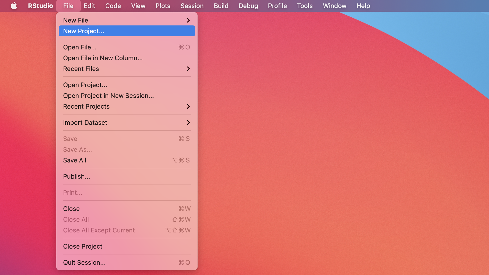
Figure 4.1: Get the R project

2. Select New Directory from the popup window.

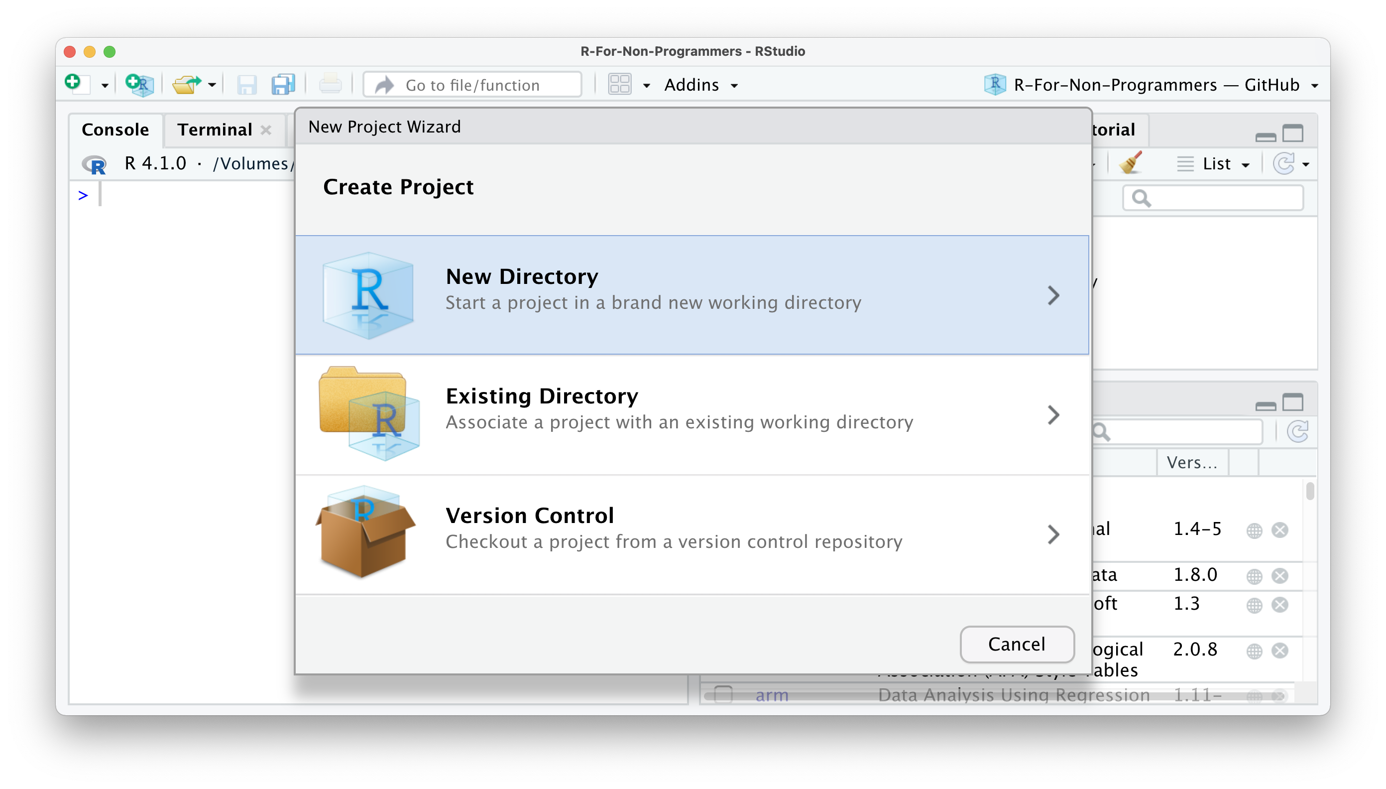
Figure 4.2: New Project Wizard pop up menu

3. Next, select New Project.

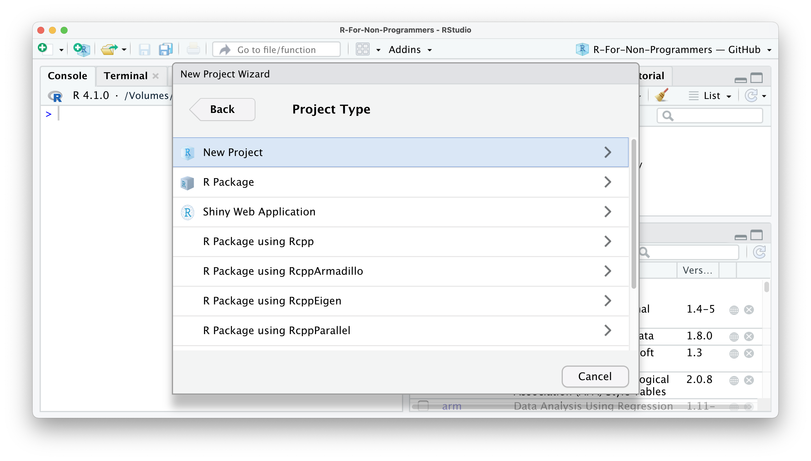
Figure 4.3: The full set of project you can initialize through the RStudio IDE

4. Pick a meaningful name for your project folder, i.e. the Directory Name. Ensure this project folder is created in the right place. You can change the subdirectory by clicking on Browse…. Ideally the subdirectory is a place where you usually store your research projects.

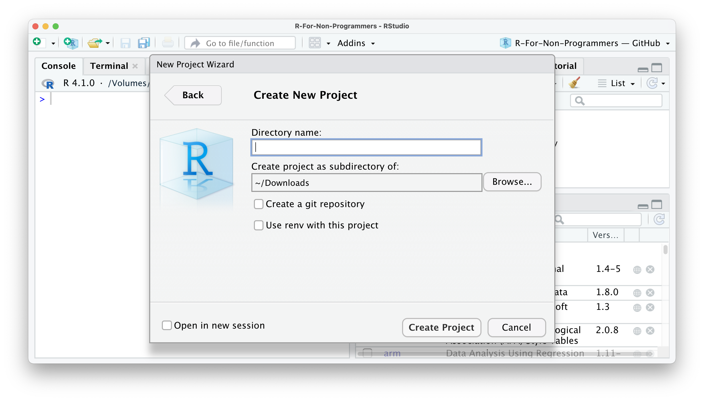
Figure 4.4: The RProject specifications

5. You have the option to Create a git repository. This is only relevant if you already have a GitHub account and wish to use version control. For now, you can happily ignore it if you do not use GitHub.

6. Lastly, tick Open in new session. This will open your R Project in a new RStudio window.

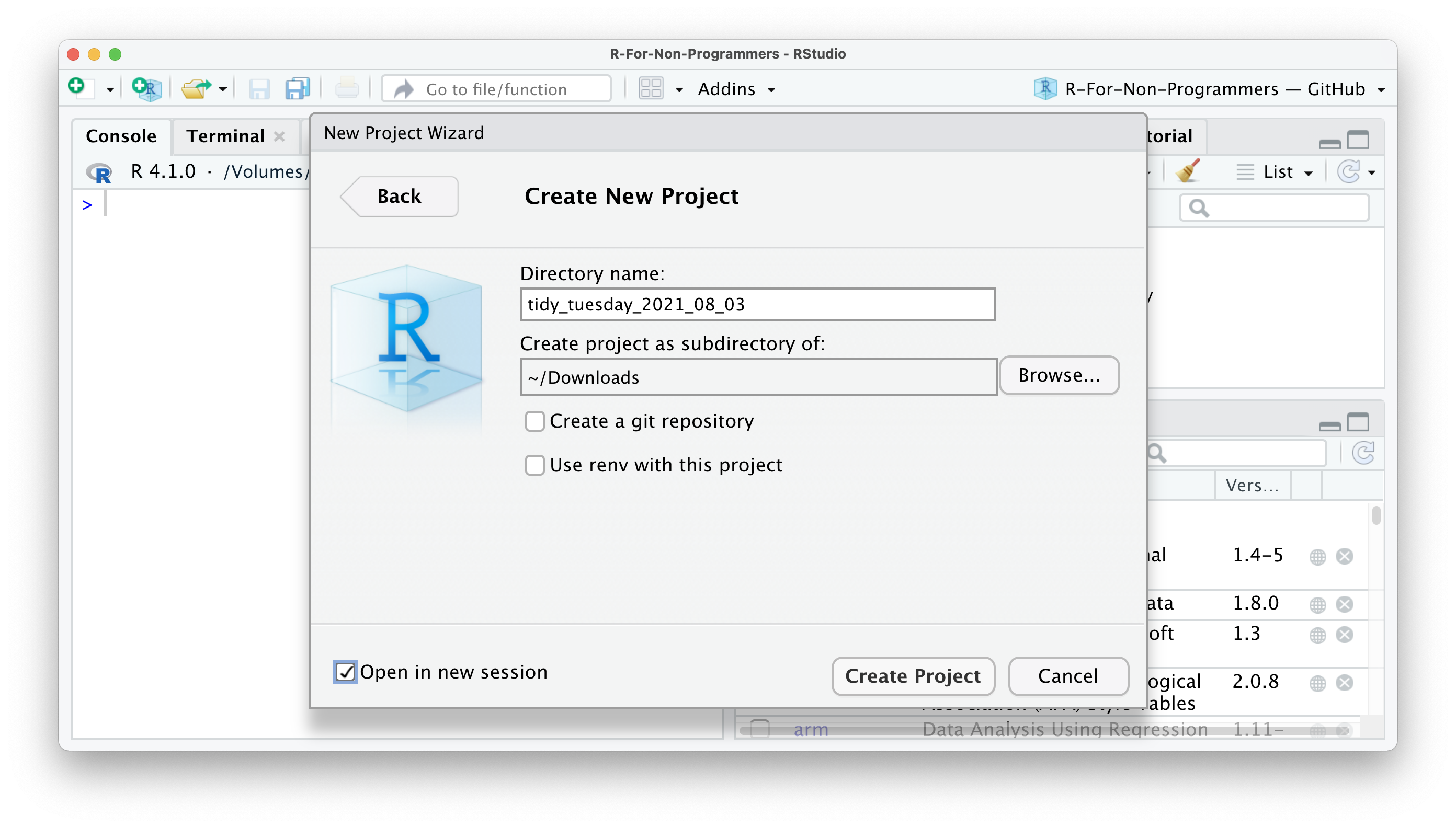
Figure 4.5: Choose a directory name for your new project

7. Once you are happy with your choices, you can click Create Project. This will open a new R Session, and you can start working on your project.

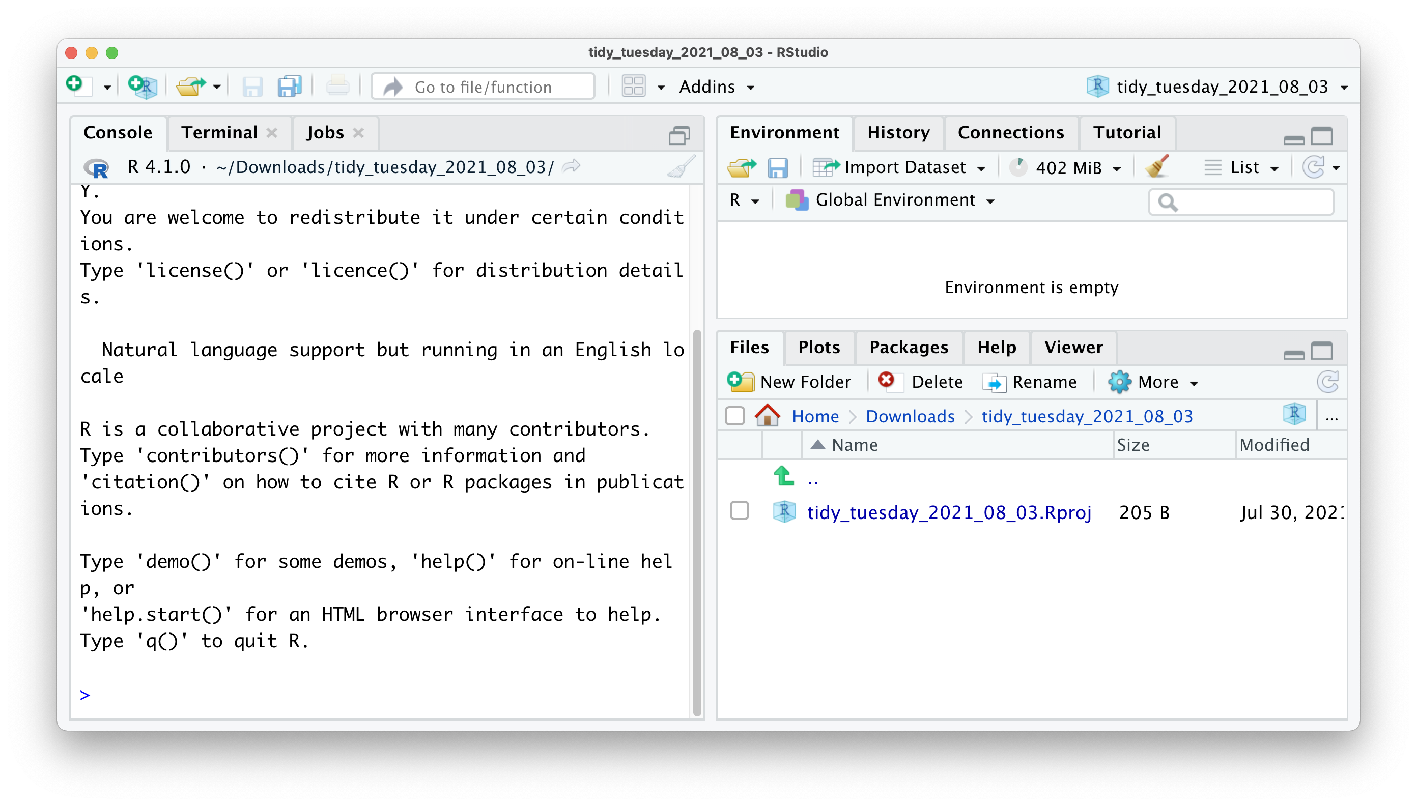
Figure 4.6: A new RStudio Session will pop up just like magic!

If you look carefully, you can see that your RStudio is now ‘branded’ with your project name. At the top of the window, you see the project name, the files pane shows the root directory where all your files will be, and even the console shows on top the file path of your project. You could set all this up manually, but I would not recommend it, not the least because it is easy and swift to work with R Projects

4.3 Working Directory with here

When you bootstrap your RProject in that way, RStudio is going to take care of many headaches that any fresher and sophmore developer have in the beginning. As a matter of fact each time you double click on the RStudio project file (the one that finishes with .RProj) RStudio will link itself to the directory on your computer you specified during the creation of the project, in the previous case “tidy_tuesday_2021_08_03”. This is called the Working Directory. What it is interesting it that this place is where R will look for files when you attempt to load them, and it is where R will save files when you save them. The location of your working directory will vary on different computers. There is a base (rather vintage) way to look for the working directory. To understrand which directory R is using as your working directory, run:

getwd()
## "/Users/niccolo/Desktop/r_projects/sbd_22-23"

However since we live in 2022 we are going to use a very convenient package i.e. here that does exactly the same thing but prettier and more intuitively.

install.packages("here")
library(here)
here()
## "/Users/niccolo/Desktop/r_projects/sbd_22-23"

here() is going to look for the .RProj file and will the Working Directory exactly where it is placed.

4.4 Creating an R Script

Code may easily grow lengthy and complicated. As a result, writing it on the console is inconvenient. As an alternative, we may write code into a R Script. An R Script is a document that is recognized by RStudio as R programming code. Non-R Script files, such as .txt,.rtf, or .md, can also be opened in RStudio, but any code typed in them will not be immediately recognized.

When you open or create a new R script, it will appear in the Source pane. This window is sometimes referred to as the ‘script editor’. An R script begins with an empty file. Good coding etiquette requires us to put a comment # on the first line to describe what this file does. Here’s a ‘TidyTuesday’ R Project sample.

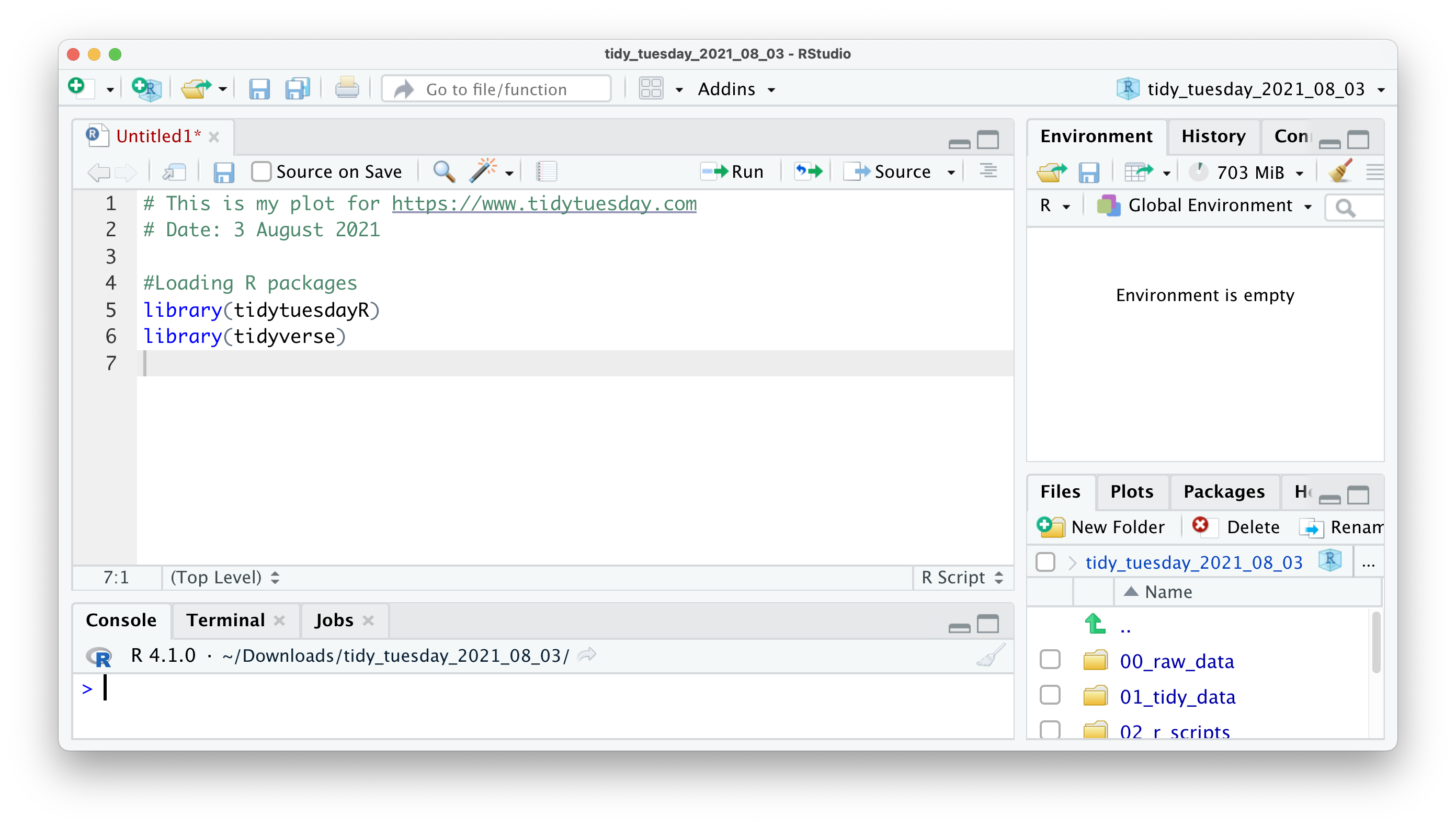
Figure 4.7: Open an R Script and write some on it

All of the examples in this tutorial are made to be copied and pasted into your own R script. However, you will need to install the R packages for certain code. Let’s give it a shot with the following code. The plot produced by this code displays which car company provides the most fuel-efficient vehicles. This code should be copied and pasted into your R script.

library(tidyverse)
mpg %>% 
  ggplot(aes(x = reorder(manufacturer, desc(hwy), FUN = median),
                   y = hwy,
                   fill = manufacturer)) +
  geom_boxplot() +
  coord_flip() +
  theme_minimal() +
  xlab("Manufacturer") +
  ylab("Highway miles per gallon")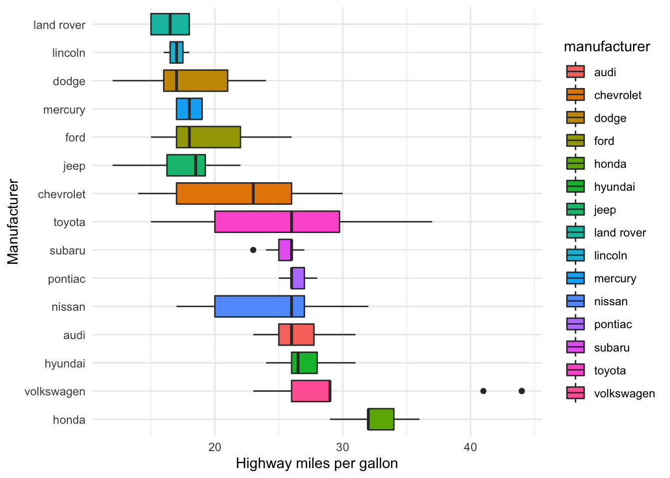

You’re probably wondering what happened to your plot. Copying the code will not execute it in your R script. However, this is required in order to develop the plot. If you pressed Return ↵, you would just add a new line. Instead, choose the code you wish to run and hit Ctrl+Return ↵ (PC) or Cmd+Return ↵ (Mac). You may also use the Run command at the top of your source window, but the keyboard shortcut is far more convenient. Furthermore, you will rapidly remember this shortcut because we will need to utilize it frequently. If everything is in order, you should see the following:

As you can see, Honda automobiles appear to travel the furthest with the same quantity of fuel (a gallon) as other vehicles. As a result, if you’re seeking for cheap automobiles, you now know where to look at.

It’s worth noting that the R script editor includes some handy features for developing code. You’ve undoubtedly noticed that part of the code we’ve pasted is blue and others is green. Because they have a distinct significance, these colors aid in making your code more understandable. In the default settings, green represents any value in ““, which often represents characters. Syntax highlighting refers to the automatic coloring of our programming code.

4.5 Using R Markdown

There is too lot to say about R Markdown, so I’ll just mention that it exists and highlight one feature that could persuade you to use it instead of plain R scripts: They appear to be Word documents (almost).

R Markdown files, as the name implies, are a mix of R scripts and ‘Markdown.’ ‘Markdown’ is a method of composing and formatting text documents without the use of software such as Microsoft Word. You instead write everything in plain text. Such plain text may be translated into a variety of document forms, including HTML webpages, PDF files, and Word documents. I recommend checking out the R Markdown Cheatsheet to learn how it works. Click File > New File > R Markdown to create a R Markdown file.

An R Markdown file is the inverse of a R script. By default, a R script treats everything as code, and we can only use language to describe what the code does by commenting #. This is what you’ve seen in all of the previous code examples. An R Markdown file, on the other hand, treats everything as text and requires us to declare what is code. We may accomplish this by injecting ‘code chunks.’ As a result, using comments # in R Markdown files is less necessary because you may write about it. Another advantage of R Markdown files is that the results of your analysis are shown immediately underneath the code chunk rather than in the terminal. They are also sometimes called notebooks since they can display both code and text together, the Python equivalent for those that have been someway exposed to Python scripting in Jupyter